MIRAGE-e Baseline #

MIRAGE-e’s baseline is basically an implementation of MaGE model macroeconomic projections. The following variables are used from MaGE’s output, the EconMap database:

GDP projections
Population
Skilled and unskilled labor
Savings rate and current account
Energy productivity

In addition to these variables from MaGE/EconMap, the following assumptions are also included in the baseline:

Fossil energy prices trajectories are calibrated after International Energy Agency projections
Sector decomposition of TFP growth between agriculture, manufacturing ans services

General presentation of the baseline design #

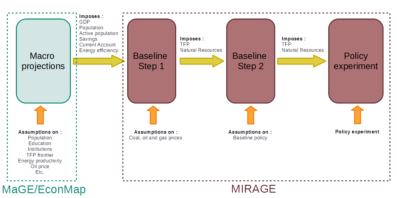
The simulation workflow with 2-step baseline

By default, the baseline exercise is made of two sets of model simulations:

Step 1 : Only projections in macroeconomic determinants. It is also possible to include in this step other assumptions, but this requires that such assumptions are not likely to significantly impact GDP growth.
- This is the “baseline” strico-sensu, as it is common in most CGE models
- In this step, the GDP trajectory is imposed to the model in order to calibrate the trajectory of TFP growth
Step 2 : Other assumptions are implemented in the second step (e.g. large free trade agreements, Paris agreement)
- This step takes the productivity calibrated in step 1 as given, and let GDP be endogenous.
- This allows to account for the effect of baseline assumptions on GDP and energy prices

GDP projections #

TFP in MIRAGE-e #

TFP in MIRAGE-e consists in a region-specific TFP, $TFP_{r,t}$ and a sector-specific component $TFPJ_{j,r,t}$. Both concern only energy and the five factors (capital, skilled labor, unskilled labor - embodied in the $VAQL_{j,r,t}$ bundle - as well as land and natural resources) of the production function:

$$ \begin{array}{rl} VAQL_{j,r,t} &= a^{VAQL}_{j,r} VA_{j,r,t} \left(TFP_{r,t}TFPJ_{j,r,t}\right)^{\sigma_{VAQL}-1} \left(\frac{P^{VA}_{j,r,t}}{P^{VAQL}_{j,r,t}}\right)^{\sigma_{VAQL}}\\\\\\ Land_{j,r,t} &= a^{Land}_{j,r} VA_{j,r,t} \left(TFP_{r,t}TFPJ_{j,r,t}\right)^{\sigma_{VAQL}-1} \left(\frac{P^{VA}_{j,r,t}}{P^{Land}_{j,r,t}}\right)^{\sigma_{VAQL}}\\\\\\ NatRes_{j,r,t}RESV_{j,t} &= a^{NatRes}_{j,r} VA_{j,r,t} \left(TFP_{r,t}TFPJ_{j,r,t}\right)^{\sigma_{VAQL}-1} \left(\frac{P^{VA}_{j,r,t}}{P^{NatRes}_{j,r,t}}\right)^{\sigma_{VAQL}} \end{array} $$

Calibration in the baseline exercise #

MIRAGE-e baseline (in Step 1) exercise starts from the following assumptions in order to calibrate a baseline trajectory for TFP:

MaGE GDP growth rates $g^{GDP}_{r,t}$
Exogenous agricultural TFP $TFP^{Agri}_{j,r,t}$
Constant 2 p.p. growth difference between manufacturing and services $\Delta g^{TFP}_j$

This translates in the following relations:

$$ \begin{array}{rll} GDP[{r,t} &= \left(1+g^{GDP}_{r,t}\right) GDP]{.underline}{r,t-1} &\\ TFP_{r,t}TFPJ_{j,r,t} &= TFP^{Agri}_{j,r,t} &\text{if}\quad j\in Agri\\ TFP_{r,t}TFPJ_{j,r,t} &= \left(1+\Delta g^{TFP}_j\right) TFP_{j,r,t} TFPJ_{j,r,t-1} &\text{if}\quad j\notin Agri \end{array} $$

Population and labor #

Population and labor by educational level are simply following the growth rate from EconMap:

$$ \begin{array}{rl} Pop\_ag_{r,t} &= ActivePopulation_{r,t}\\ TotalUnSkL_{r,t} &= TotalUnSkL_{r,t-1} \left(1+g^{UnSkL}_{r,t}\right)\\ TotalSkL_{r,t} &= TotalSkL_{r,t-1} \left(1+g^{SkL}_{r,t}\right) \end{array} $$

Savings rate and current account #

Current Account in MIRAGE-e #

Current account (im)balances $CABal_{s,t}$ are used in the macroeconomic closure equation:

$$ Sav_{s,t} REV_{s,t} = P^{INVTOT}_{s,t} INVTOT_{s,t} + CABal_{s,t} WGDPVal_t $$

Calibration of savings rate and current account #

Savings rate #

Savings rate follows EconMap projections $Savings_{r,t}$ additively:

$$ Sav_{r,t} = Sav_{r,t-1} + \left(Savings_{r,t}-Savings_{r,t-1}\right) $$

Current account #

Current account imbalances evolve additively:

$$ CABal_{r,t} = CABal_{r,t-1} + \delta CABal_{r,t} $$

while $\delta CABal_{r,t}$ is calibrated after EconMap’s $CurrentAccount_{r,t}$, but keeping world current account balance:

$$ \begin{array}{lr} \delta CABal^0_{r,t} = CurrentAccount_{r,t} \frac{GDP[{r,t}}{\sum_sGDP]{.underline}{s,t}} - CurrentAccount_{r,t-1} \frac{GDP[{r,t-1}}{\sum_sGDP]{.underline}{s,t-1}}\\\\\\ \delta CABal_{r,t} = \delta CABal^0_{r,t} - \left(\sum_s \delta CABal^0_{s,t}\right) \frac{GDP[{r,t}}{\sum_sGDP]{.underline}{s,t}} \end{array} $$

Energy productivity #

<alert type=“info” icon=“glyphicon glyphicon-asterisk”>This feature is only available if energy in value added is toggled on</alert>

Energy productivity in MIRAGE-e #

In MIRAGE-e, total energy consumption by each sector $ETOT_{j,r,t}$ is subject to energy-specific technological improvement $EE_{j,r,t}$:

$$ ETOT_{j,r,t} = a^E_{j,r,t} EE_{j,r,t} KE_{j,r,t} \left(\frac{PKE_{j,r,t}}{PE_{j,r,t}}\right)^{\sigma_{KE}} $$

$EE_{j,r,t}$ is applied to every sector, except for non-electricity energy producing sectors (coal, oil, gas, petroleum and coal products), whose energy productivity is constant.

Baseline calibration #

This energy-specific technological improvement is calibrated in the baseline after MaGE’s projected energy productivity $B_{r,t}$. However, three things differ between $B_{r,t}$ and $EE_{j,r,t}$:

In MIRAGE notations, share coefficients and productivity improvement appear in CES functions at the power of $1/\sigma$ whereas in MaGE, $B_{r,t}$ appears at the power of $(\sigma-1)/\sigma$. We therefore introduce $EProd_{r,t}$:

$$EProd_{r,t} \equiv B_{r,t}^{\sigma_{KE}-1} $$

$B_{r,t}$ is labelled in dollars per ton of oil equivalent, whereas $EE_{j,r,t}$ and $EProd_{r,t}$ are calibrated at 1

$$EProd_{j,r,t} = EProd_{j,r,t-1} \left(1+g^B_{r,t}\right)^{\sigma_{KE}-1} $$

In MaGE’s production function, $B_{r,t}$ (as well as capital-labor productivity $A_{r,t}$) include an hypothetical TFP, whereas in MIRAGE, $EE_{j,r,t}$ comes in addition to the TFP level $TFP_{r,t}TFPJ_{j,r,t}$

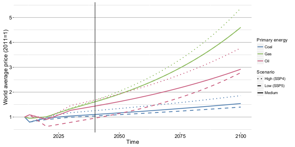
$$EE_{j,r,t} = \left(\frac{EProd_{r,t}}{TFP_{r,t}TFPJ_{j,r,t}}\right)^{\sigma_{KE}-1} $$

Fossil fuels energy prices #

Energy prices projections from World Energy Outlook 2015

Natural resources in MIRAGE-e #

In MIRAGE-e, a sector-specific reserve factor $RESV_j,t$ is introduced to scale natural resources globally for each primary fossil energy (coal, oil gas)[(the equation is provided here for perfect competition only)]:

$$ NatRes_{i,r,t} RESV_{i,t} = a^{NatRes}_{i,r} Y_{i,r,t} \left(\frac{P^Y_{r,t}}{P^{NatRes}_{r,t}}\right)^{\sigma^{NatRes}} $$

Calibration of natural resources in the baseline #

During the baseline exercise, the reserve factor is set endogenous, while world price defined as:

$$ \log \left(PWORLD_{i,t}PWO_i\right) = \frac{\sum_{r,s} TRADE_{i,r,s,t} \log PCIF_{i,r,s,t}}{\sum_{r,s} TRADE_{i,r,s,t}} $$

is kept exogenous:

$$ PWORLD_{i,t} = PWORLD_{i,t-1} \left(1+g^{P}_{i,t}\right) $$