Final demand (1.1) #

General approach #

In each region, a representative agent allocates a fixed share of the regional income to savings and purchases goods for final consumption with the rest of the income. The saving rates follow projections by EconMap. The utility function of this agent is intra-temporal.

The representative agent gathers government and final consumers, meaning that they share the same demand function. Hence, the representative agent both pays and earns taxes. Furthermore, no public budget constraint has to be taken into account explicitly: this constraint is implicit to meet the representative agent’s budget constraint. As a consequence, unless otherwise indicated (modelling a distorsive replacement tax does not raise any technical problem), any decrease in tax revenues (for example as a consequence of a trade liberalisation) is compensated by a non-distorsive replacement tax. However, the magnitude of the losses in tax revenues is an interesting information, provided in standard result tables.

The LES-CES function #

Utility function

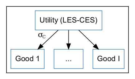
We consider that final per capita consumption follows a nesting of CES and LES demand functions. This extension of LES to the slightly more flexible framework of the CES was first proposed by [(:harvard:Pollak71)]. This LES-CES can be expressed by the following program

$$ \max U = \left[\sum_i \alpha_i^{1/\sigma} (C_i - \bar{c_i}^{(\sigma-1)/\sigma})\right]^{\sigma/(\sigma-1)} $$

subject to $\sum_i P_iC_i=I$. The consumer demands for each sector $i$ an incompressible level $\bar{c}_{i}$. She allocates the remaining part of her income $I$ according to the CES demand function with elasticity $\sigma$. $C_{i}$ represents the consumption from sector $i$ including incompressible consumption. $P_{i}$ is the price of an unitary level of consumption.

The LES-CES function inherits from the LES function the possibility to be calibrated on any positive income elasticity. With an income growth, the LES-CES converges to a CES. Own-price elasticities are strongly linked to income elasticities: sectors with low income elasticity have a high incompressible consumption. Since most of their consumption is fixed, except for a very high elasticity of substitution in the CES nest, these sectors have a low own-price elasticity. Finally, regularity requires that income be superior to the cost of subsistence $\sum_{i}P_{i}\bar{c}_{i}$.

Calibration of utility parameters #

Data #

Utility parameters (minimal consumption level, elasticity of substitution) are calibrated using elasticities available on the website of the United States Department of Agriculture (USDA). The download page gathers several files: a zip-file including elasticities (of income and of prices) for 1996 and Excel files for 2005. More precisely, two datasets are needed: (i) compensated own-price elasticity for broad consumption and (ii) unconditional own-price elasticity for food subcategories. Estimates cover 114 and 144 countries for 1996 and 2005 respectively. For details on how these elasticities are obtained, please refer to the USDA documentation.

LES-CES can only accommodate positive income elasticities, so we change all negative income elasticities to a very low value, namely 0.025.

Calibration procedure #

All the parameters are calibrated at the same time using an optimization procedure that minimizes the discrepancies between target and calibrated own-price elasticities, subject to the respect of the initial consumption and the income elasticities. The calibration is done on the consumption per capita. There are usually several solutions that minimise the objective (same final own-price elasticities, but different set of parameters), depending on the initial values. These multiple solutions correspond to the same initial behavior but to different behavior after a change in prices or income.

For each country, the calibration that uses as target the own price elasticity follows the program

$$\min_{\sigma_{i},0 \le \bar{c}_{i} \le C_{i}^{t}, \alpha_{i}} \sum_{i} \frac{P_{i} C_{i}^{t}}{I}\left(e_{ii}-e_{ii}^{t}\right)^{2} $$

Subject to

$$ C_{i}^{t}=Pop_{i} \left[\bar{c}_{i}+\frac{\alpha_{i}\left(I-\gamma\right)}{Pop_{i} P}\left(\frac{P}{P_{i}}\right)^{\sigma_{i}}\right] $$

$$ e_{ii}=-\frac{\alpha_i}{C_i^{t}}\left(\frac{P}{P_i}\right)^{\left(\sigma_{i}-1\right)}\left[C_i^{t}+\sigma_{i}\left(\bar{c}_i-C_i^{t}+\frac{I-\gamma}{P_i}\right)\right] $$

with $e_{ii}^{t}$ is the target uncompensated own-price elasticity (this is only for illustration, we use the type of own-price elasticity corresponding to the elasticities sources), $C_{i}^{t}$ is the target consumption level (from the GTAP database), $\gamma = \sum_i P_i\bar{c}_i$ and $P=\left(\sum_i \alpha_iP_i^{1-\sigma}\right)^{\frac{1}{1-\sigma}}$.

According to the source availability, the calibration is also done targeting the income elasticity $\eta_{i}$, with

$$ \eta_{i}^{t} = \frac{\alpha_iI}{P_iC_i^{t}}\left(\frac{P}{P_i}\right)^{\sigma_{i}-1} $$