MIRAGE-e Baseline

For MIRAGE-e and the versions that follow it, the dynamic baseline follows the macroeconomic projections of MaGE model. The following variables are used from MaGE’s output, the EconMap database:

• GDP projections
• Population
• Skilled and unskilled labor
• Savings rate and current account
• Energy productivity

In addition to these variables from MaGE/EconMap, the following assumptions are also included in the baseline:

• Fossil energy prices trajectories are calibrated after International Energy Agency projections
• Sector decomposition of TFP growth between agriculture, manufacturing, and services

General presentation of the baseline design

The simulation workflow with 2-step baseline

By default, the baseline exercise is made of two sets of model simulations:

1. Only projections in macroeconomic determinants. It is also possible to include in this step other assumptions, but this requires that such assumptions are not likely to impact GDP growth significantly.
   • This is the “baseline” strico-sensu, as it is common in most CGE models
   • In this step, the GDP trajectory is imposed on the model in order to calibrate the trajectory of TFP growth
2. Other assumptions are implemented in the second step (e.g. large free trade agreements, Paris Agreement)
   • This step takes the productivity calibrated in step 1 as given, and let GDP be endogenous.
   • This allows us to account for the effect of baseline assumptions on GDP and energy prices

GDP projections

TFP in MIRAGE-e

TFP in MIRAGE-e consists in a region-specific TFP, \(TFP_{r,t}\) and a sector-specific component \(TFPJ_{j,r,t}\). Both concern only energy and the five factors (capital, skilled labor, unskilled labor - embodied in the \(VAQL_{j,r,t}\) bundle - as well as land and natural resources) of the production function: \[ \begin{array}{rl} VAQL_{j,r,t} &= a^{VAQL}_{j,r} VA_{j,r,t} \left(TFP_{r,t}TFPJ_{j,r,t}\right)^{\sigma_{VAQL}-1} \left(\frac{P^{VA}_{j,r,t}}{P^{VAQL}_{j,r,t}}\right)^{\sigma_{VAQL}}\\\\\\ Land_{j,r,t} &= a^{Land}_{j,r} VA_{j,r,t} \left(TFP_{r,t}TFPJ_{j,r,t}\right)^{\sigma_{VAQL}-1} \left(\frac{P^{VA}_{j,r,t}}{P^{Land}_{j,r,t}}\right)^{\sigma_{VAQL}}\\\\\\ NatRes_{j,r,t}RESV_{j,t} &= a^{NatRes}_{j,r} VA_{j,r,t} \left(TFP_{r,t}TFPJ_{j,r,t}\right)^{\sigma_{VAQL}-1} \left(\frac{P^{VA}_{j,r,t}}{P^{NatRes}_{j,r,t}}\right)^{\sigma_{VAQL}} \end{array} \]

Calibration in the baseline exercise

MIRAGE-e baseline (in Step 1) exercise starts from the following assumptions in order to calibrate a baseline trajectory for TFP:

• MaGE GDP growth rates: \(g^{GDP}_{r,t}\)
• Exogenous agricultural TFP: \(TFP^{Agri}_{j,r,t}\)
• Constant 2 p.p. growth difference between manufacturing and services: \(\Delta g^{TFP}_j\)

This translates into the following relations: \[ \begin{array}{rll} GDP_{r,t} &= \left(1+g^{GDP}_{r,t}\right) GDP_{r,t-1} &\\ TFP_{r,t}TFPJ_{j,r,t} &= TFP^{Agri}_{j,r,t} &\text{if}\quad j\in Agri\\ TFP_{r,t}TFPJ_{j,r,t} &= \left(1+\Delta g^{TFP}_j\right) TFP_{j,r,t} TFPJ_{j,r,t-1} &\text{if}\quad j\notin Agri \end{array} \]

Population and labor

Population and labor by educational level simply follow the growth rate from EconMap: \[ \begin{array}{rl} Pop\_ag_{r,t} &= ActivePopulation_{r,t}\\ TotalUnSkL_{r,t} &= TotalUnSkL_{r,t-1} \left(1+g^{UnSkL}_{r,t}\right)\\ TotalSkL_{r,t} &= TotalSkL_{r,t-1} \left(1+g^{SkL}_{r,t}\right) \end{array} \]

Savings rate and current account

Current account in MIRAGE-e

Current account (im)balances \(CABal_{s,t}\) are used in the macroeconomic closure equation:

\[ Sav_{s,t} REV_{s,t} = P^{INVTOT}_{s,t} INVTOT_{s,t} + CABal_{s,t} WGDPVal_t \]

Calibration of savings rate and current account

Savings rate

Savings rate follows EconMap projections \(Savings_{r,t}\) additively: \[ Sav_{r,t} = Sav_{r,t-1} + \left(Savings_{r,t}-Savings_{r,t-1}\right)\]

Current account

Current account imbalances evolve additively: \[ CABal_{r,t} = CABal_{r,t-1} + \delta CABal_{r,t}\]

while \(\delta CABal_{r,t}\) is calibrated after EconMap’s \(CurrentAccount_{r,t}\), but keeping world current account balance: \[ \begin{array}{lr} \delta CABal^0_{r,t} = CurrentAccount_{r,t} \frac{GDP[{r,t}}{\sum_s GDP_{s,t}} - CurrentAccount_{r,t-1} \frac{GDP[{r,t-1}}{\sum_s GDP_{s,t-1}}\\\\\\ \delta CABal_{r,t} = \delta CABal^0_{r,t} - \left(\sum_s \delta CABal^0_{s,t}\right) \frac{GDP[{r,t}}{\sum_s GDP_{s,t}} \end{array} \]

Energy productivity

This feature is only available if energy in value added is toggled on.

Energy productivity in MIRAGE-e

In MIRAGE-e, total energy consumption by each sector \(ETOT_{j,r,t}\) is subject to energy-specific technological improvement \(EE_{j,r,t}\): \[ETOT_{j,r,t} = a^E_{j,r,t} EE_{j,r,t} KE_{j,r,t} \left(\frac{PKE_{j,r,t}}{PE_{j,r,t}}\right)^{\sigma_{KE}}\]

\(EE_{j,r,t}\) is applied to every sector except for non-electricity energy-producing sectors (coal, oil, gas, petroleum, and coal products), whose energy productivity is constant.

Baseline calibration

This energy-specific technological improvement is calibrated in the baseline after MaGE’s projected energy productivity \(B_{r,t}\). However, three things differ between \(B_{r,t}\) and \(EE_{j,r,t}\):

• In MIRAGE notations, share coefficients and productivity improvement appear in CES functions at the power of \(1/\sigma\) whereas in MaGE, \(B_{r,t}\) appears at the power of \((\sigma-1)/\sigma\). We therefore introduce \(EProd_{r,t}\): \[EProd_{r,t} \equiv B_{r,t}^{\sigma_{KE}-1}\]
• \(B_{r,t}\) is labeled in dollars per ton of oil equivalent, whereas \(EE_{j,r,t}\) and \(EProd_{r,t}\) are calibrated at 1 \[EProd_{j,r,t} = EProd_{j,r,t-1} \left(1+g^B_{r,t}\right)^{\sigma_{KE}-1}\]
• In MaGE’s production function, \(B_{r,t}\) (as well as capital-labor productivity \(A_{r,t}\)) include a hypothetical TFP, whereas in MIRAGE, \(EE_{j,r,t}\) comes in addition to the TFP level \(TFP_{r,t}TFPJ_{j,r,t}\) \[EE_{j,r,t} = \left(\frac{EProd_{r,t}}{TFP_{r,t}TFPJ_{j,r,t}}\right)^{\sigma_{KE}-1}\]

Fossil fuels energy prices

Energy prices projections from World Energy Outlook 2015

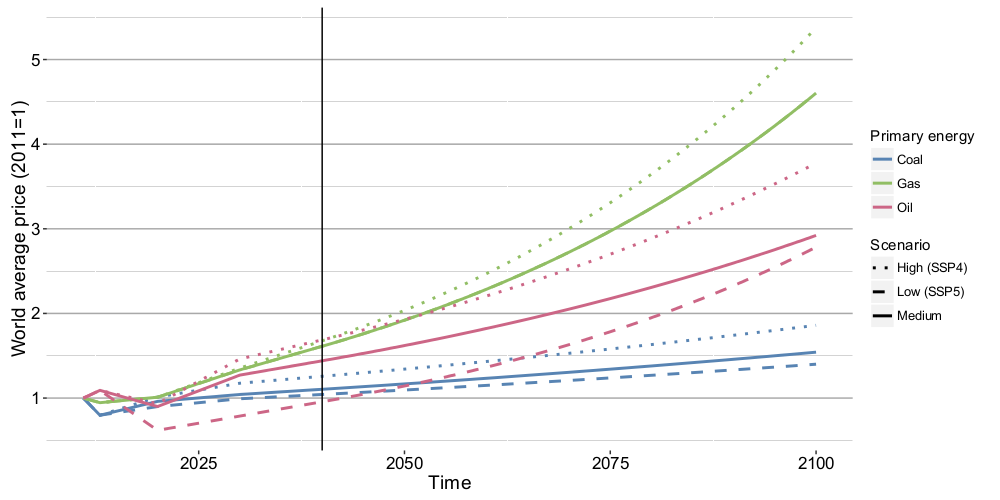
Natural resources in MIRAGE-e

In MIRAGE-e, a sector-specific reserve factor \(RESV_{j,t}\) is introduced to scale natural resources globally for each primary fossil energy, coal, oil gas (the equation is provided here for perfect competition only): \[NatRes_{i,r,t} RESV_{i,t} = a^{NatRes}_{i,r} Y_{i,r,t} \left(\frac{P^Y_{r,t}}{P^{NatRes}_{r,t}}\right)^{\sigma^{NatRes}}\]

Calibration of natural resources in the baseline

During the baseline exercise, the reserve factor is set endogenous, while world price is defined as: \[ \log \left(PWORLD_{i,t}PWO_i\right) = \frac{\sum_{r,s} TRADE_{i,r,s,t} \log PCIF_{i,r,s,t}}{\sum_{r,s} TRADE_{i,r,s,t}} \] is kept exogenous: \[ PWORLD_{i,t} = PWORLD_{i,t-1}\left(1+g^{P}_{i,t}\right).\]